Data leakage in ML for biological and clinical data: what it is and how to avoid it

When we build machine learning models on biological or clinical data, data leakage is one of the fastest ways to get results that look amazing on paper and fail spectacularly in reality.

Informally, leakage means your model sees information during training or validation that it will not see at deployment time. This can happen through patient overlap between train and test, normalisation that looks at all samples at once, features that encode the label, or outcome-dependent filtering of the dataset.

This post explains leakage in a maths-first way, but each concept is also tied to a mental picture or plot you can use to recognise and avoid it.

1. Formalising data leakage

Suppose we want to learn a model $f_\theta$ that predicts an outcome $Y$ from input $X$. In the ideal setting we assume:

\[(X, Y) \sim P_\text{deploy}(X, Y) \quad\text{and}\quad \theta^\star = \arg\min_\theta \; \mathbb{E}_{(X,Y)\sim P_\text{deploy}}[\mathcal{L}(f_\theta(X), Y)].\]

In practice, we only have a finite dataset $\mathcal{D} = {(x_i, y_i)}_{i=1}^n$, and we estimate performance by splitting into train/validation/test sets. Data leakage occurs when our training or validation process uses extra variables $Z$ that:

are correlated with $Y$ in the dataset we have, but
will not be available, or will have a different distribution, at deployment.

Mathematically, the training-time joint distribution involves $Z$:

\[(X, Z, Y) \sim P_\text{train}(X, Z, Y),\]

but at deployment we only see $X$:

\[(X, Y) \sim P_\text{deploy}(X, Y) = \sum_{z} P_\text{train}(X, Z=z, Y).\]

If the model learns to depend on $Z$ (directly or indirectly), our empirical risk estimate

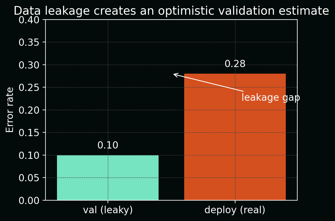
\[\hat{R}_\text{val} = \frac{1}{|\mathcal{D}_\text{val}|} \sum_{(x_i, y_i)\in\mathcal{D}_\text{val}} \mathcal{L}(f_\theta(x_i, z_i), y_i)\]

will be optimistically biased relative to the true deployment risk (R_\text{deploy}).

The figure below shows this as a simple bar chart: apparent validation error (\hat{R}\text{val}) (low) vs true deployment error (R\text{deploy}) (higher), with the difference highlighted as the leakage gap.

Bar chart showing optimistic validation error vs higher deployment error due to leakage

2. Sample-level vs patient-level splits

In biological and clinical data, we rarely have IID points. Instead, we often have groups (patients, donors, wells, slides, time‑series) and multiple samples per group:

\[\{(x_{ij}, y_{ij})\}_{j=1}^{n_i} \quad \text{for patient } i = 1,\dots,M.\]

If we randomly split at the sample level, we may end up with:

training set: some tiles from patient $i$,
test set: other tiles from the same patient $i$.

Then the conditional distributions differ:

\[P_\text{train}(X \mid \text{patient}=i) \approx P_\text{test}(X \mid \text{patient}=i),\]

even though at deployment we care about:

\[P_\text{deploy}(X, Y) = \sum_{i} P(X, Y \mid \text{patient}=i)\,P(\text{patient}=i),\]

with entirely new patients.

This artificially inflates performance because the model can learn patient‑specific fingerprints (batch, staining, scanner, genetics) rather than general biological patterns.

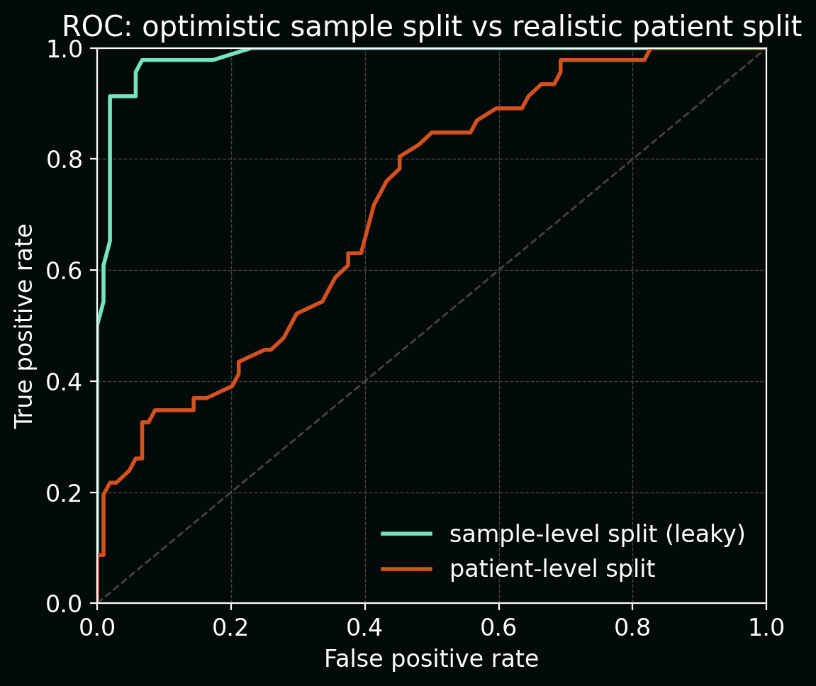
The plot below compares ROC curves for the same model under two splitting schemes:

random sample-level split (optimistic AUC close to 1.0), vs
true patient-level split (lower, more realistic AUC).

ROC curves for sample-level vs patient-level data splits

3. Normalisation and preprocessing leakage

Many pipelines apply operations of the form:

\[T(x_i; \mathcal{D}) = \frac{x_i - \mu(\mathcal{D})}{\sigma(\mathcal{D})},\]

where $\mu(\mathcal{D})$ and $\sigma(\mathcal{D})$ are estimated from the full dataset (train + validation + test). This is a classic leakage pattern:

the transform $T$ for a test point depends on other test points and all of train,
at deployment we will not have access to future test data to recompute $T$.

The leakage‑safe version uses training-only statistics:

\[T_\text{train}(x_i) = \frac{x_i - \mu(\mathcal{D}_\text{train})}{\sigma(\mathcal{D}_\text{train})},\]

and applies the same $T_\text{train}$ to validation/test and deployment data.

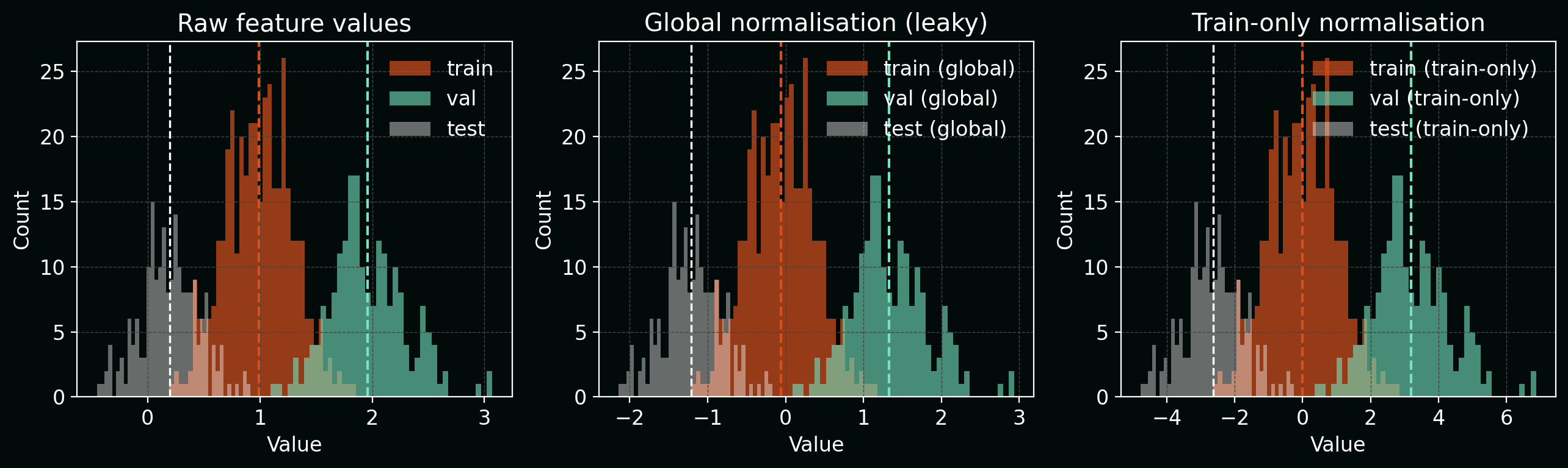
The figure below shows histograms of a single feature:

before normalisation,
after “global” normalisation (leaky, using all data), and
after train‑only normalisation.

The global version subtly centres and rescales each split differently, which bakes test‑set information into the transform.

Histograms showing global vs train-only normalisation and their effect on feature distributions

The same principle applies to:

PCA / UMAP fits,
feature selection,
imputation of missing values,
batch-effect correction.

All of these must be fitted only on training data, then applied to held‑out data.

4. Label leakage: using future or outcome-derived information

Label leakage happens when a feature is a function of the outcome $Y$ or of future information that would not be known at prediction time.

Example: predicting hospital mortality $Y \in {0,1}$ with features including:

\[X = \big(\text{vitals at admission}, \text{lab values in first 24h}, \text{discharge disposition}\big).\]

Here, “discharge disposition” is (almost) a deterministic function of the outcome—if the patient died, the discharge code encodes that. The mutual information

\[I(Y; X_\text{discharge}) = H(Y) - H(Y \mid X_\text{discharge})\]

is close to its maximum, so the model can trivially recover $Y$ from this feature.

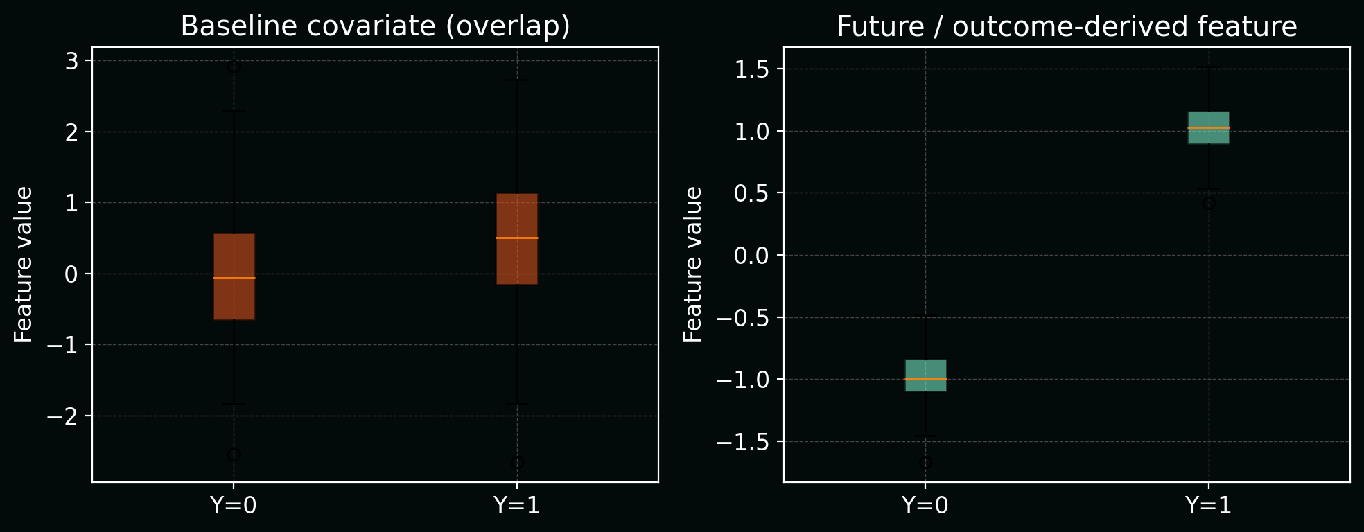
Below, a simple boxplot shows how this “future” feature almost perfectly separates the two outcome classes, unlike realistic baseline covariates which overlap heavily.

Boxplot showing a future feature that almost perfectly separates outcome classes

Mitigation:

define a time-of-decision (t_0),
only include features measured at or before (t_0),
drop or carefully model any variables that are functions of the outcome.

5. Outcome-dependent dataset construction

Sometimes leakage is baked into how the dataset is assembled.

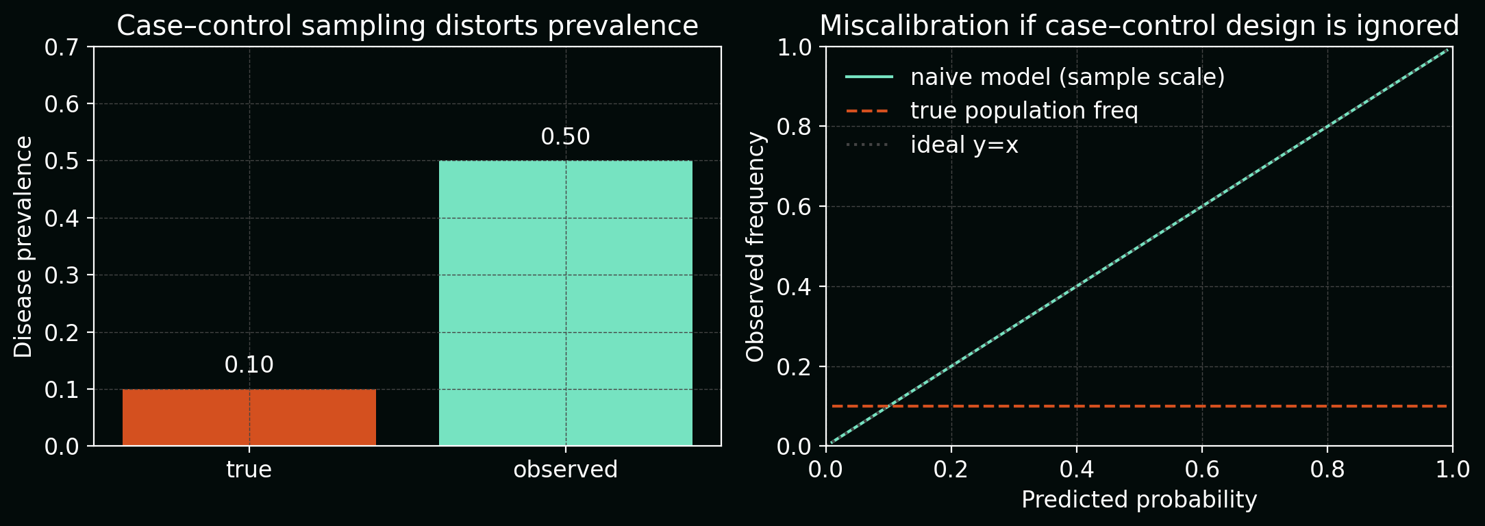
Example: in a case–control design, you might:

pull all positive cases (e.g. disease present),
then randomly sample a subset of negatives.

If the sampling probabilities (\pi(y)) depend on (y), then the observed label distribution satisfies:

\[P_\text{obs}(Y=y) \propto \pi(y)\,P_\text{true}(Y=y),\]

and naïve estimates of prevalence or calibration will be biased.

In extreme cases, you might filter images based on post‑hoc manual review that depends on seeing the outcome, effectively encoding hints about (Y) into inclusion/exclusion.

The next figure combines two views:

a bar chart comparing true disease prevalence vs observed prevalence in the case–control sample, and
a calibration curve showing over‑confident predictions if you ignore the sampling scheme.

True vs observed prevalence and resulting miscalibration in a case-control design

Mitigation:

explicitly model the sampling process (e.g. inverse‑probability weighting),
when possible, construct train/validation/test splits before outcome‑dependent filtering.

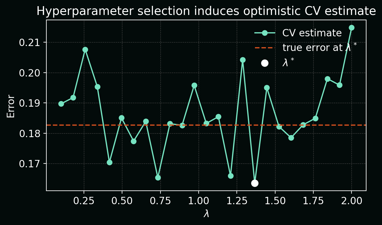
6. Cross-validation and hyperparameter tuning leakage

In (K)-fold cross‑validation, we often evaluate a model family ({f_{\theta,\lambda}}) over hyperparameters (\lambda). Leakage arises if we:

Use cross‑validation both to select (\lambda^\star) and to report the “final” performance.
Accidentally let folds share patients (as in Section 2).

Mathematically, if we define:

\[\hat{R}_k(\lambda) = \frac{1}{|\mathcal{D}_k^\text{val}|}\sum_{(x_i, y_i)\in\mathcal{D}_k^\text{val}} \mathcal{L}(f_{\theta_k(\lambda)}(x_i), y_i),\]

and pick

\[\lambda^\star = \arg\min_\lambda \frac{1}{K}\sum_{k=1}^{K} \hat{R}_k(\lambda),\]

then simply reporting

\[\hat{R}_\text{CV}(\lambda^\star)\]

as “the” performance underestimates the true error due to selection bias.

In the plot below, each point is a CV estimate (\hat{R}_\text{CV}(\lambda)) for one hyperparameter value; (\lambda^\star) is the minimum. A horizontal line shows that the true error at (\lambda^\star) is higher than the minimum CV estimate.

Cross-validation error vs hyperparameter, highlighting optimistic bias at the selected lambda

Mitigation:

Use cross‑validation only for model selection, not for the final number.
Treat CV error as a tool for choosing the hyperparameter region (or model family). Once you have chosen (\lambda^\star), retrain on all training data with (\lambda^\star) and then evaluate exactly once on a held‑out test set to get the number you quote.
Define folds at the patient/slide/batch level, not per‑sample.
When you construct (\mathcal{D}_k^\text{train}) and (\mathcal{D}_k^\text{val}), group by the natural entities in your data (patients, slides, plates, donors), and ensure no entity appears in more than one fold. This prevents optimistic performance due to the same patient contributing examples to multiple folds.

7. Consequences of leakage: why it really matters

Leakage doesn’t just make your metrics look a bit too good—it changes what your model learns. If (\tilde{X}) includes leaky features and (X) is the real deployable feature set, your trained model approximates:

\[f_\theta(\tilde{X}) \approx \mathbb{E}[Y \mid \tilde{X}],\]

but what you actually need in deployment is:

\[f^\star(X) = \mathbb{E}[Y \mid X].\]

When (\tilde{X}) carries extra information about (Y) that (X) does not, we can have:

\[I(Y; \tilde{X}) \gg I(Y; X),\]

where (I(\cdot;\cdot)) is mutual information. The model appears highly predictive in offline evaluation but loses that signal in the real‑world feature space.

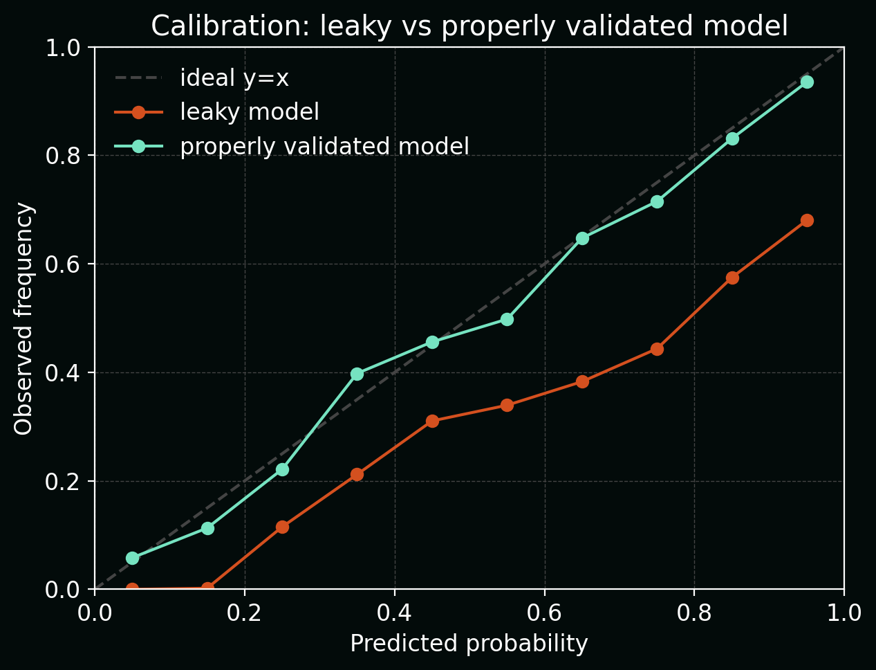
The calibration plot below contrasts a leaky model (sharply over‑confident: predicted probabilities cluster near 0 or 1, but observed frequencies sit closer to 0.5) with a properly validated model that tracks the diagonal much more closely.

Calibration curves comparing an over-confident leaky model with a properly validated model

In biology/clinical settings, this can lead to:

incorrect scientific conclusions (e.g. over‑claiming predictive biomarkers),
wasted experimental validation,
dangerous decisions if models are pushed toward clinical deployment.

8. Practical mitigation checklist

To make leakage less likely in your own pipelines, it helps to turn vague “best practices” into concrete checks you can run against each project:

Define your deployment scenario explicitly.
Before touching any code, write down: who the model will make predictions for, when those predictions happen in the workflow, and which variables are available at that time. If a feature would only be known later (e.g. discharge code, follow‑up measurements), do not include it in training features, even if it is convenient and strongly predictive.
Split by entity, not by sample.
Decide what the atomic unit is in your setting (patient, donor, animal, plate, slide, well, field‑of‑view, time‑series) and ensure each unit appears in exactly one of train/validation/test. For example, in histopathology you might group tiles by slide; in longitudinal EHR data you might group visits by patient ID and split on patient IDs.
Fit transforms on train only, then freeze them.
Any operation that “learns” from the data—normalisation, PCA, feature selection, imputation, batch correction—must be fitted on (\mathcal{D}_\text{train}) and then applied as a fixed transform to validation and test. In code, this usually means calling .fit or .fit_transform on train only, and .transform on val/test, never refitting on the full dataset before evaluation.
Keep a locked‑box test set and touch it once.
Reserve a test set at the very beginning and keep it out of sight during model development. Use cross‑validation and the validation set for all model and hyperparameter decisions; only after you have frozen the full pipeline (including preprocessing and thresholds) should you evaluate on the test set to obtain the performance numbers you share externally.
Audit your features for proxies and future information.
For every column in your design matrix, ask: could this be (directly or indirectly) a proxy for the label? or does it depend on information that would only be available after the prediction time? Drop, censor, or carefully model any features that fail this test (e.g. outcome‑coded variables, post‑treatment measurements, identifiers that encode site or assay batch).

If you’d like, we can follow up with a concrete worked example (e.g. predicting response from baseline imaging and labs) where we build a leaky model on purpose, visualise how it fails, and then fix the leakage step‑by‑step.