Random Forests vs Gaussian Processes: A Practical Maths-First Comparison

Random Forests and Gaussian Processes (GPs) are both powerful non‑parametric models (models that don’t fix a single, limited functional form in advance) for regression and classification, but they come from very different mathematical worlds.

Random Forests [1] live in the land of decision trees, bagging, and majority votes. Here, bagging [2] (“bootstrap aggregation”) just means training many models on resampled versions of the data and averaging them to reduce variance. Gaussian Processes [3] live in the land of kernel functions, multivariate Gaussians, and Bayesian inference. A kernel function measures similarity between two inputs and controls how strongly information is shared between nearby points, and Bayesian inference is the process of starting from a prior belief, then updating it with data to obtain a posterior distribution over model parameters or functions.

In this post I’ll directly compare:

• The underlying maths
• How they model functions
• Pros and limitations in practice, especially for scientific modelling.

---

1. What problem are we solving?

We assume we have $n$ data points ${(x_i, y_i)}_{i=1}^n$, where

• $x_i \in \mathbb{R}^d$ is a $d$-dimensional feature vector (e.g. descriptors of a molecule, experimental conditions, simulation parameters),
• $y_i \in \mathbb{R}$ is a scalar response (e.g. binding energy, yield, diffusion constant).

We want to learn a function $f(x)$ such that

\[y_i = f(x_i) + \varepsilon_i,\]

where $\varepsilon_i$ is noise. Both Random Forests and Gaussian Processes try to approximate this $f$, but they do it in fundamentally different ways.

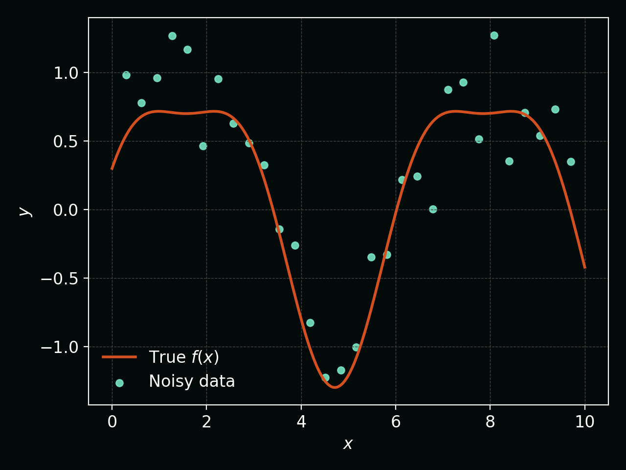
To visualise this, the figure below shows a smooth underlying function (orange curve) and noisy observations (teal points) that we use to infer it:

---

2. Random Forests: Piecewise-constant ensembles

2.1 Single decision tree

A regression tree recursively partitions input space into regions ${R_m}_{m=1}^M$. Within each region $R_m$, the prediction is just a constant, typically the mean of the targets in that region:

\[\hat{f}_{\text{tree}}(x) = \sum_{m=1}^{M} c_m \, \mathbb{I}(x \in R_m),\]

where

• $R_m$ are disjoint regions defined by axis-aligned splits (e.g. $x_j \le t$),
• $c_m = \frac{1}{\lvert R_m\rvert} \sum_{i: x_i \in R_m} y_i$ is the average label in region $m$,
• $\mathbb{I}(\cdot)$ is an indicator function.

A single tree is high‑variance: small changes in the data can change the splits a lot.

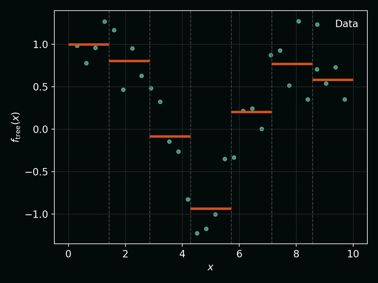
Below, the vertical dashed lines show the regions $R_m$ and the orange steps show the piecewise‑constant tree prediction:

2.2 Bagging and Random Forests

A Random Forest [1] averages many such trees built on bootstrapped data with extra randomness in feature selection.

For regression, if we build $T$ trees and the $t$-th tree predicts $\hat{f}_t(x)$, the forest prediction is:

\[\hat{f}_{\text{RF}}(x) = \frac{1}{T} \sum_{t=1}^{T} \hat{f}_t(x).\]

Key mathematical points:

• Bagging (bootstrap aggregation) [2] reduces variance: \(\mathrm{Var}\big[\hat{f}_{\text{RF}}(x)\big] \approx \rho \, \sigma^2 + \frac{1 - \rho}{T} \sigma^2,\) where $\sigma^2$ is the variance of a single tree and $\rho$ is the correlation between trees. Random feature selection aims to decrease $\rho$.

• The resulting function is piecewise constant, though averaging many trees can create a “staircase” that approximates smooth functions surprisingly well.

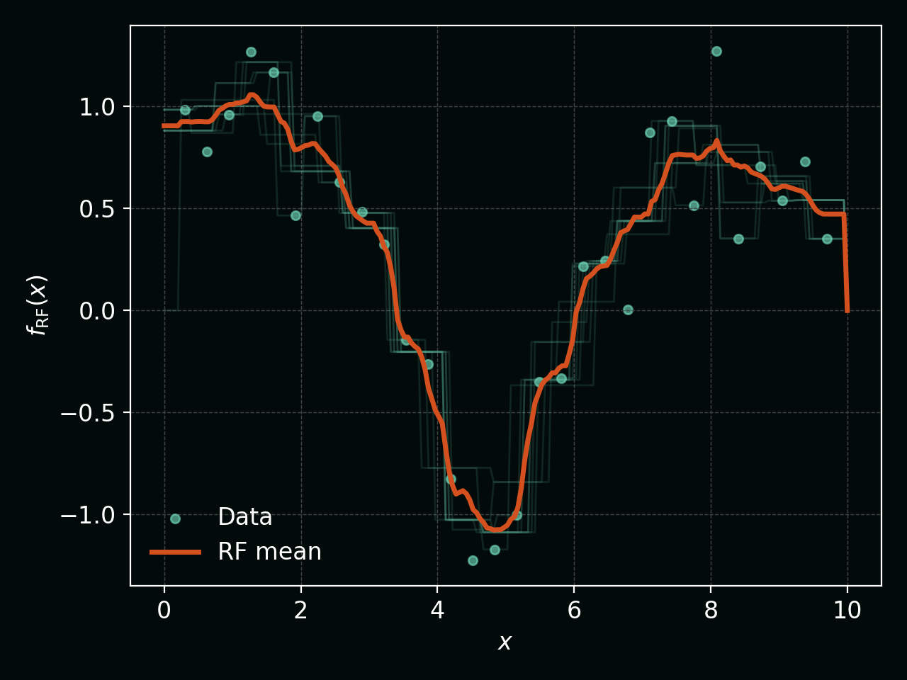
The next figure shows several individual tree predictions (faint teal) and their Random Forest average (thick orange), illustrating how averaging smooths out the individual rough trees:

2.3 Random Forest “uncertainty”

Random Forests do not have a clean probabilistic model by default. A common heuristic for uncertainty in regression is the sample variance of tree predictions [5]:

\[\widehat{\mathrm{Var}}_{\text{RF}}(x) = \frac{1}{T-1} \sum_{t=1}^{T} \Big(\hat{f}_t(x) - \hat{f}_{\text{RF}}(x)\Big)^2.\]

This is not a fully Bayesian posterior variance, but in practice it behaves like an “empirical uncertainty”: high where trees disagree, low where they agree.

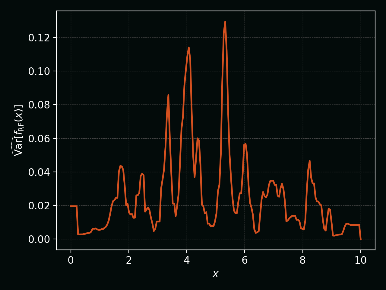
The empirical uncertainty can be visualised by plotting this variance as a function of $x$:

---

3. Gaussian Processes: Functions as infinite-dimensional Gaussians

Gaussian Processes start from a very different philosophy: instead of explicitly building basis functions or trees, we put a prior over functions.

3.1 GP prior

A Gaussian Process [3] is defined as:

\[f(x) \sim \mathcal{GP}\big(m(x), k(x, x')\big),\]

which means that for any finite collection of points $X = [x_1, \dots, x_n]$, the vector of function values

\[\mathbf{f} = \big(f(x_1), \dots, f(x_n)\big)^\top\]

follows a multivariate normal distribution:

\[\mathbf{f} \sim \mathcal{N}\left(\mathbf{m}, K\right),\]

with

• $\mathbf{m}_i = m(x_i)$,
• $K_{ij} = k(x_i, x_j)$.

Common choices:

• Zero mean $m(x) = 0$,
• Stationary kernels like the squared exponential (RBF): \(k_{\text{RBF}}(x, x') = \sigma_f^2 \exp\left( -\frac{1}{2} \sum_{j=1}^{d} \frac{(x_j - x'_j)^2}{\ell_j^2} \right),\) where $\ell_j$ are length scales and $\sigma_f^2$ is the signal variance.

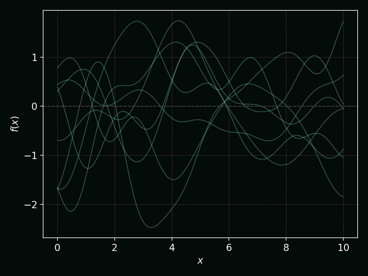
Before seeing any data, a GP prior corresponds to a distribution over smooth functions. The figure below shows several draws from a zero‑mean GP prior with an RBF kernel:

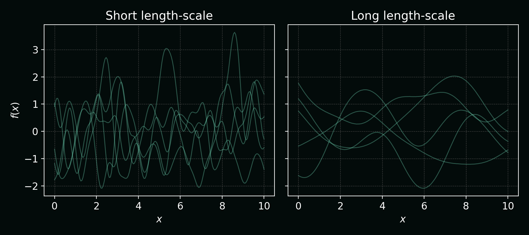
Changing the kernel length‑scale changes how wiggly those functions are. Shorter length‑scales give rougher functions; longer ones give smoother functions:

3.2 GP regression posterior

Assume a GP prior $f \sim \mathcal{GP}(0, k)$ and Gaussian noise:

\[y_i = f(x_i) + \varepsilon_i, \quad \varepsilon_i \sim \mathcal{N}(0, \sigma_n^2).\]

Let:

• $X \in \mathbb{R}^{n \times d}$ be training inputs,
• $\mathbf{y} \in \mathbb{R}^{n}$ be targets,
• $x_\ast$ be a test input.

Define:

• $K = K(X, X)$ with $K_{ij} = k(x_i, x_j)$,
• $\mathbf{k}\ast = k(X, x\ast)$ (an $n$-vector),
• $k_{\ast\ast} = k(x_\ast, x_\ast)$.

The GP posterior predictive distribution [3] is:

\[p(f_\ast \mid x_\ast, X, \mathbf{y}) = \mathcal{N}\big(\mu_\ast, \sigma_\ast^2\big),\]

with

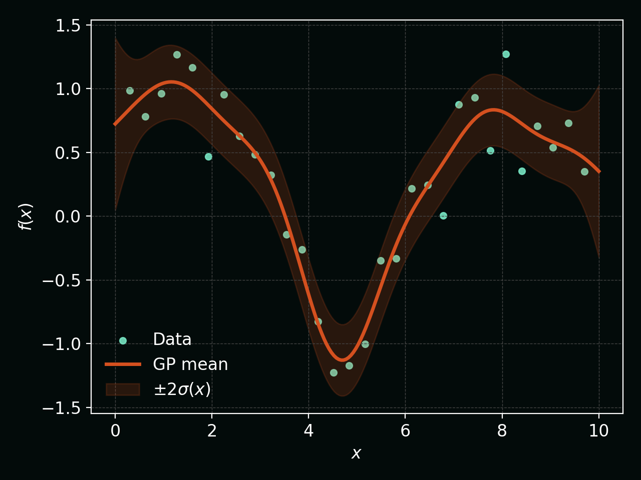
\[\mu_\ast = \mathbf{k}_\ast^\top (K + \sigma_n^2 I)^{-1} \mathbf{y},\] \[\sigma_\ast^2 = k_{\ast\ast} - \mathbf{k}_\ast^\top (K + \sigma_n^2 I)^{-1} \mathbf{k}_\ast.\]

This is where GPs shine: we get both a mean prediction and a principled posterior variance derived from a full probabilistic model.

The plot below shows the GP posterior mean (orange line) and a $\pm 2\sigma(x)$ credible band (shaded orange), together with the observed data (teal points):

3.3 Hyperparameters and marginal likelihood

The kernel has hyperparameters $\theta$ (e.g. length scales $\ell_j$, variance $\sigma_f^2$, noise $\sigma_n^2$). A standard approach is to choose $\theta$ by maximizing the log marginal likelihood [3]:

\[\log p(\mathbf{y} \mid X, \theta) = -\frac{1}{2} \mathbf{y}^\top (K_\theta + \sigma_n^2 I)^{-1} \mathbf{y} - \frac{1}{2} \log \big| K_\theta + \sigma_n^2 I \big| - \frac{n}{2} \log(2\pi).\]

This balances data fit and model complexity automatically.

---

4. Comparing the modelling philosophies

4.1 Function representation

• Random Forests:
  • Represent $f(x)$ as an average of many piecewise-constant trees.
  • No explicit smoothness prior; smoothness emerges only from averaging many rough trees.
  • Naturally handle heterogeneous features and nonlinear interactions via splits.
• Gaussian Processes:
  • Represent $f(x)$ as a sample from a prior over smooth functions defined by the kernel.
  • Smoothness, periodicity, and other structure are explicitly encoded in the kernel $k(x,x’)$.
  • You can design kernels to reflect physics/chemistry knowledge (e.g. periodic for angles, Matérn for rougher functions, sums/products for additive interactions).

4.2 Complexity control

• Random Forests:
  • Control tree depth, minimum samples per leaf, number of trees.
  • Theoretical view: bagging reduces variance but doesn’t shrink individual trees; not a Bayesian model.
• Gaussian Processes:
  • Complexity controlled by kernel hyperparameters and noise variance.
  • Bayesian framework: posterior automatically trades off data fit vs smoothness via the marginal likelihood.

---

5. Practical pros and cons

5.1 Random Forests

Pros

• Robust defaults: often work well with minimal tuning.
• Handle mixed data types (categorical, continuous) and messy feature scaling.
• Nonlinear feature interactions emerge naturally from splits.
• Training scales roughly as $O(T \cdot n \log n)$ for $T$ trees — much better than naive GP $O(n^3)$ for large $n$.
• Resistant to overfitting compared to single trees.
• Can still work surprisingly well at low sample sizes, as random forests are Highly modifiable: there are many practical extensions (e.g. quantile Random Forests [4], “honest” forests, conformal predictors, Mondrian forests) that tweak how trees are built or aggregated to give better calibrated uncertainties or tailored loss functions, which lets each region capture local trends instead of a single constant while keeping the same basic, fast training loop.

Cons For standard random forest:

• Predictions are effectively piecewise-constant; can be less smooth, which sometimes clashes with physical intuition.
• Uncertainty is heuristic (variance across trees), not a fully Bayesian posterior.
• Extrapolation outside the training domain is often poor: they tend to predict near the average of observed values.

5.2 Gaussian Processes

Pros

• Provide full predictive distributions $p(f_\ast \mid x_\ast, X, \mathbf{y})$ with principled uncertainty.
• Excellent for small‑to‑medium datasets ($n$ up to a few thousand) where data is expensive (e.g. simulations, experiments).
• Kernels allow you to encode prior knowledge:
  • Smoothness scales,
  • Periodicity,
  • Additive or multiplicative structure.
• Natural fit for Bayesian optimization [6], active learning, and design of experiments (DOE), where uncertainty matters.

Cons

• Computationally expensive: naive training and prediction scale as $O(n^3)$ and $O(n^2)$ due to matrix inversions, so wall‑clock time can become prohibitive beyond a few thousand points unless you use sparse or approximate GP variants [7, 8].
• Kernel choice and hyperparameter tuning matter a lot; can be harder to “just use” than Random Forests.
• Handling high‑dimensional, heterogeneous, or categorical data is more awkward.

---

6. When to prefer which?

Choose Random Forests when:

• You have many samples ($n \gtrsim 10^4$) and moderate feature dimensionality.
• You want a strong baseline with minimal tuning.
• Feature types are mixed or messy, and you want a model that “just works”.
• You care more about point prediction accuracy than about calibrated uncertainties.

Choose Gaussian Processes when:

• Data is expensive (simulations or experiments) and $n$ is small to medium.
• You need uncertainty-aware decisions:
  • Bayesian optimization [6],
  • Adaptive experiments,
  • Active learning.
• You have domain knowledge you can encode into kernels (e.g. “this function should be smooth on this length scale”).
• Smooth interpolation and physically plausible behaviour between data points matter more than raw accuracy on massive datasets.

---

7. Summary

Mathematically, Random Forests and Gaussian Processes are almost opposites:

• Random Forests: frequentist, ensemble of piecewise-constant trees, variance reduction through bagging, heuristic uncertainty.
• Gaussian Processes: Bayesian, prior over smooth functions, exact Gaussian posterior, principled uncertainty at every point.

In scientific and engineering settings, a good workflow is often:

1. Start with a Random Forest as a fast baseline and for feature importance.
2. Switch to a Gaussian Process when:
   • You narrow down to a smaller, more carefully designed dataset, and
   • You want uncertainty‑aware modelling, Bayesian optimization, or interpretable smooth behaviour.

Both tools are valuable; the right one depends on whether you care more about speed and robustness at scale (Random Forests) or probabilistic, uncertainty‑aware modelling of expensive data (Gaussian Processes).

---

References

1. Breiman, L. (2001). Random Forests. Machine Learning, 45(1), 5-32. https://doi.org/10.1023/A:1010933404324

2. Breiman, L. (1996). Bagging Predictors. Machine Learning, 24(2), 123-140. https://doi.org/10.1007/BF00058655

3. Rasmussen, C. E., & Williams, C. K. I. (2006). Gaussian Processes for Machine Learning. MIT Press. https://gaussianprocess.org/gpml/

4. Meinshausen, N. (2006). Quantile Regression Forests. Journal of Machine Learning Research, 7, 983-999.

5. Wager, S., Hastie, T., & Efron, B. (2014). Confidence Intervals for Random Forests: The Jackknife and the Infinitesimal Jackknife. Journal of Machine Learning Research, 15, 1625-1651.

6. Frazier, P. I. (2018). A Tutorial on Bayesian Optimization. arXiv preprint arXiv:1807.02811.

7. Hensman, J., Matthews, A., & Ghahramani, Z. (2015). Scalable Variational Gaussian Process Classification. Proceedings of the Eighteenth International Conference on Artificial Intelligence and Statistics, 351-360.

8. Quinonero-Candela, J., & Rasmussen, C. E. (2005). A Unifying View of Sparse Approximate Gaussian Process Regression. Journal of Machine Learning Research, 6, 1939-1959.